How To Draw Phase Portraits Of Linear Systems

Show Mobile Find Show All NotesHide All Notes

Mobile Notice

Y'all appear to be on a device with a "narrow" screen width (i.e. you are probably on a mobile telephone). Due to the nature of the mathematics on this site it is best views in landscape mode. If your device is non in landscape mode many of the equations will run off the side of your device (should be able to whorl to run into them) and some of the carte items volition be cut off due to the narrow screen width.

Section 5-half-dozen : Stage Plane

Before proceeding with actually solving systems of differential equations there's one topic that we demand to accept a wait at. This is a topic that's not e'er taught in a differential equations class but in case you're in a course where it is taught we should cover it so that you are prepared for it.

Let's start with a general homogeneous organisation,

\[\begin{equation}\vec x' = A\vec x\label{eq:eq1}\end{equation}\]

Discover that

\[\vec x = \vec 0\]

is a solution to the system of differential equations. What we'd like to ask is, practise the other solutions to the organization approach this solution as \(t\) increases or practice they motility abroad from this solution? We did something similar to this when we classified equilibrium solutions in a previous department. In fact, what we're doing here is simply an extension of this idea to systems of differential equations.

The solution \(\vec x = \vec 0\) is called an equilibrium solution for the system. As with the single differential equations instance, equilibrium solutions are those solutions for which

\[A\vec x = \vec 0\]

We are going to assume that \(A\) is a nonsingular matrix and hence will accept merely 1 solution,

\[\vec x = \vec 0\]

and and so we will have only i equilibrium solution.

Back in the unmarried differential equation case think that we started past choosing values of \(y\) and plugging these into the function \(f(y)\) to determine values of \(y'\). We so used these values to sketch tangents to the solution at that item value of \(y\). From this we could sketch in some solutions and use this information to classify the equilibrium solutions.

We are going to do something similar here, only it will be slightly different too. First, nosotros are going to restrict ourselves downwards to the \(2 \times ii\) case. So, we'll be looking at systems of the form,

\[\begin{array}{*{20}{c}}\begin{align*}{{x'}_1} & = a{x_1} + b{x_2}\\ {{x'}_2} & = c{x_1} + d{x_2}\end{marshal*}&{\hspace{0.25in} \Rightarrow \hspace{0.25in}\hspace{0.25in}\vec x' = \left( {\begin{array}{*{20}{c}}a&b\\c&d\end{array}} \right)\vec x}\end{array}\]

Solutions to this system will exist of the form,

\[\vec x = \left( {\brainstorm{array}{*{twenty}{c}}{{x_1}\left( t \right)}\\{{x_2}\left( t \right)}\cease{array}} \correct)\]

and our single equilibrium solution volition exist,

\[\vec ten = \left( {\begin{array}{*{20}{c}}0\\0\end{assortment}} \right)\]

In the unmarried differential equation case nosotros were able to sketch the solution, \(y(t)\) in the y-t plane and come across bodily solutions. However, this would somewhat difficult in this case since our solutions are actually vectors. What we're going to practise here is call up of the solutions to the system as points in the \({x_1}\,{x_2}\) airplane and plot these points. Our equilibrium solution will represent to the origin of \({x_1}\,{x_2}\). aeroplane and the \({x_1}\,{x_2}\) plane is called the phase plane.

To sketch a solution in the phase aeroplane we can pick values of \(t\) and plug these into the solution. This gives united states of america a point in the \({x_1}\,{x_2}\) or phase plane that nosotros can plot. Doing this for many values of \(t\) will then requite us a sketch of what the solution will exist doing in the phase plane. A sketch of a detail solution in the phase plane is chosen the trajectory of the solution. One time nosotros have the trajectory of a solution sketched we tin can then enquire whether or non the solution will approach the equilibrium solution as \(t\) increases.

We would like to be able to sketch trajectories without actually having solutions in mitt. There are a couple of ways to do this. We'll look at 1 of those here and we'll look at the other in the next couple of sections.

I manner to get a sketch of trajectories is to do something similar to what nosotros did the kickoff time we looked at equilibrium solutions. We tin choose values of \(\vec 10\) (note that these will be points in the phase plane) and compute \(A\vec 10\). This volition requite a vector that represents \(\vec x'\)at that item solution. As with the single differential equation case this vector will exist tangent to the trajectory at that bespeak. Nosotros can sketch a bunch of the tangent vectors and and then sketch in the trajectories.

This is a fairly work intensive way of doing these and isn't the way to do them in general. However, it is a way to get trajectories without doing whatsoever solution work. All nosotros need is the system of differential equations. Let's take a quick look at an case.

Example 1 Sketch some trajectories for the system, \[\begin{assortment}{*{20}{c}}\brainstorm{marshal*}{{ten'}_1} & = {x_1} + 2{x_2}\\ {{ten'}_2} & = three{x_1} + 2{x_2}\end{align*}&{\hspace{0.25in} \Rightarrow \hspace{0.25in}\vec 10' = \left( {\begin{assortment}{*{20}{c}}one&2\\3&ii\terminate{array}} \right)\vec x}\cease{array}\]

Show Solution

So, what we need to exercise is pick some points in the stage airplane, plug them into the right side of the system. Nosotros'll do this for a couple of points.

\[\brainstorm{align*}\vec x & = \left( {\begin{array}{*{20}{c}}{ - 1}\\one\end{array}} \right) & \Rightarrow \hspace{0.25in}\vec ten'& = \left( {\begin{array}{*{twenty}{c}}i&two\\3&2\end{assortment}} \right)\left( {\begin{array}{*{20}{c}}{ - 1}\\1\cease{array}} \right) = \left( {\begin{assortment}{*{20}{c}}ane\\{ - 1}\stop{array}} \right)\\ \vec x & = \left( {\begin{array}{*{20}{c}}ii\\0\end{assortment}} \correct) & \Rightarrow \hspace{0.25in}\vec ten' & = \left( {\begin{array}{*{20}{c}}one&ii\\3&2\end{assortment}} \right)\left( {\begin{array}{*{xx}{c}}2\\0\end{array}} \right) = \left( {\begin{array}{*{twenty}{c}}2\\half-dozen\end{array}} \right)\hspace{0.25in}\\ \vec x & = \left( {\begin{array}{*{20}{c}}{ - 3}\\{ - ii}\end{array}} \correct) & \Rightarrow \hspace{0.25in}\vec ten' & = \left( {\begin{array}{*{20}{c}}1&2\\iii&2\terminate{array}} \right)\left( {\begin{array}{*{20}{c}}{ - iii}\\{ - 2}\end{array}} \correct) = \left( {\begin{array}{*{20}{c}}{ - 7}\\{ - xiii}\end{array}} \right)\hspace{0.25in}\end{align*}\]

So, what does this tell u.s.? Well at the signal \(\left( { - 1,1} \right)\) in the phase airplane in that location will be a vector pointing in the direction \(\left\langle {one, - 1} \correct\rangle \). At the point \(\left( {two,0} \right)\) there volition be a vector pointing in the direction \(\left\langle {ii,half dozen} \correct\rangle \). At the point \(\left( { - three, - 2} \right)\) there will be a vector pointing in the direction \(\left\langle { - vii, - thirteen} \correct\rangle \).

Doing this for a large number of points in the stage airplane will give the following sketch of vectors.

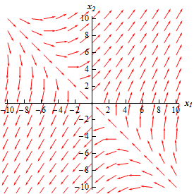
Now all we need to do is sketch in some trajectories. To do this all we need to do is remember that the vectors in the sketch higher up are tangent to the trajectories. As well, the management of the vectors give the direction of the trajectory as \(t\) increases so nosotros tin can bear witness the time dependence of the solution by adding in arrows to the trajectories.

Doing this gives the following sketch.

This sketch is called the phase portrait. Usually phase portraits simply include the trajectories of the solutions and not any vectors. All of our phase portraits form this point on will only include the trajectories.

In this case it looks like well-nigh of the solutions will first away from the equilibrium solution then as \(t\) starts to increase they move in towards the equilibrium solution and so eventually outset moving away from the equilibrium solution again.

There seem to exist iv solutions that have slightly unlike behaviors. It looks like two of the solutions will start at (or virtually at least) the equilibrium solution and then motion direct abroad from information technology while two other solutions start away from the equilibrium solution and then move directly in towards the equilibrium solution.

In these kinds of cases we call the equilibrium bespeak a saddle point and we telephone call the equilibrium signal in this instance unstable since all merely two of the solutions are moving abroad from it as \(t\) increases.

As we noted earlier this is non by and large the way that we will sketch trajectories. All we really need to go the trajectories are the eigenvalues and eigenvectors of the matrix \(A\). We will meet how to do this over the next couple of sections as we solve the systems.

Here are a few more phase portraits so you can see some more possible examples. Nosotros'll actually be generating several of these throughout the course of the next couple of sections.

Non all possible phase portraits have been shown here. These are here to bear witness y'all some of the possibilities. Make sure to notice that several kinds can be either asymptotically stable or unstable depending upon the direction of the arrows.

Notice the difference betwixt stable and asymptotically stable. In an asymptotically stable node or spiral all the trajectories will move in towards the equilibrium point every bit t increases, whereas a center (which is always stable) trajectory will just movement around the equilibrium point just never actually move in towards it.

Source: https://tutorial.math.lamar.edu/classes/de/phaseplane.aspx

Posted by: charettebegather1962.blogspot.com

Share this post